Business Analysis
Overview
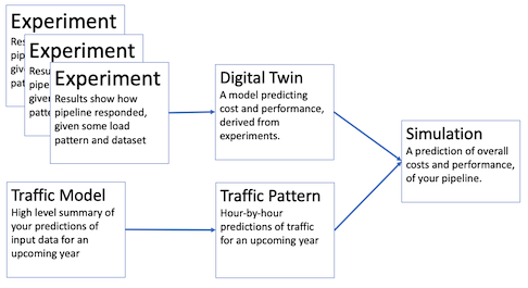
This set of PlantD resources lets you lay out a prediction of what inbound traffic will look like for a year of operation, with its seasonal or daily highs and lows, and estimate the total cost, overall performance. You can now extrapolate from experiments to assess the business implications of using the pipeline.
Regular Flow: Digital Twin constructed from user-defined experiments
Schema Aware Flow: Digital Twin triggers creation of an appropriate set of experiments
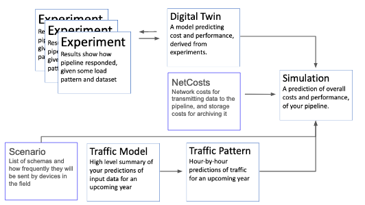
The business analysis has two operation modes, "regular" and "schema aware".
In the "regular mode", if you have run one or more experiments on a pipeline, you can now extrapolate from those experiments. This mode assumes the pipeline is fed by a single, stable, mix of data schemas, and only attempts to model variation in the total quantity of data.
In the "schema aware" mode, the digital twin will automatically create a set of experiments that test how the pipeline reacts differently with a different mix of schemas; it uses linear regression to generalize how a pipeline will react to new mixes of schemas in the future. In this mode, after the experiments are run, the modeler can create a "scenario" specifying a new mix of schemas, and run simulations predicting pipeline performance, without needing to rerun experiments.
Additionally, in schema-aware mode, a "Net Costs" object may be specified, which additionally predicts network and storage costs in the simulation, based on the raw amount of traffic coming in to the system.
Experiment
To run an analysis, you should start by conducting Experiments. In principle, many experiments with different mixes of dataset contents and load patterns can expose a variety of pipeline behaviors, which the Digital Twin can use to construct an accurate model.
If you want to vary the mix of schemas in your simulation, the digital twin will create the experiments for you.
Digital Twin
The digital twin summarizes a set of experiments, mathematically, to describe the likely cost, latency, and throughput of a pipeline given a fluctuating load level.
Note that the digital twin CANNOT process a real dataset, just a time series describing the SIZE of a dataset. If your pipeline behaves differently depending on the content of the data, the digital twin cannot capture that.
As an open source project, you can of course create more sophisticated analyses of experiments to produce more advanced twins; but out of the box we provide the following kinds of twin:
-
simple analyzes the first experiment in the list, assumes that the load pattern exceeds the pipeline's throughput capabilities, and thus uses the maximum throughput as the pipeline's peak. The model it builds assumes the pipeline cannot scale beyond this, but has an infinite queue to handle load faster than that throughput. It assumes cost does not depend on the load, just on the length of time the pipeline is running.
-
quickscaling uses the simple model as a base, but assumes an optimal horizontal scaling algorithm. Thus latency is never affected by queuing, but cost is proportional to the number of instances necessary to handle any given amount of load.
If you are building a schema-aware Digital Twin, that is, one that behaves differently depending on which data schemas are more prevalent in the input, then choose "schemaaware" as the twin type. If you do this, you will also need to supply the following:
- dataset should be the name and namespace of an existing dataset that has been tested to work with the pipeline. When you save the twin object, it will use this dataset to create a set of experiments that borrow schemas from this dataset, but vary in their quantities.
- maximum rps limits the total quantity of data that these new experiments will send to the pipeline. Choose something 50-70 percent higher than what you believe the pipeline can handle. The exact quantity doesn't matter too much. If the pipeline autoscales to handle any quantity, this simulation will not work well -- you'll need to modify the business analysis code to add more sophisticated experimental analysis to build a specialized simulation.
Traffic Model
The traffic model is a set of parameters abstractly describing the load a pipeline will face over some projected future year. There is currently no GUI to create this model; you must download a JSON file, edit or replace it manually or using your own scripts, then upload a replacement.
The parameters are as follows:
start_row_cnt: The average number of records per second received at the start of the year, ignoring daily and monthly variationsyearly_growth_rate: By what factor is traffic expected to grow or shrink over the course of the year? For example 1.0 means no overall change despite monthly and weekly variation; 0.5 would mean an overall shrinkage of data ingestion by 50%.model_name: You can safely ignore this; it can be used to represent the provenance of your data; however this is not the name used by PlantD; it's for your own documentation purposes. The name used by PlantD is specified in the user interface.corrections_monthly: For each month of the year, a correction factor reflecting how much higher or lower traffic will be that month compared to the average. 1.0 means a typical month; 1.5 means 50% more traffic than usual. These twelve numbers should average to 1.0. The format of this array is a json record, with fields:data: a comma-separated list of 12 valuesindex: a comma-separated list of the numbers from 1 to 12, representing corresponding monthsindex_name: the name of this index,Monthname: the name of this data series,row_cnt_seasonal_correction
corrections_hourly: For each hour of a week, a similar correction factor reflecting how much higher or lower traffic will be at that hour of the typical week. The format of this array is a json record, with fields:data: a comma-separated list of 168 values (i.e. 24 hours x 7 days)index: a comma-separated list of lists of day-hour pairs:[["FRI", 0], ["FRI", 1], ["FRI", 2],...the order doesn't matter as long as they align with the dataindex_names: a list containing the names of the two indexes,["DOW", "Hour"]
Traffic Pattern
This is an internal object not visible to the user -- it is an hour by hour prediction of input load, generated by working out the implications of the Traffic Model.
Note that in the case of a Schema Aware simulation with a Scenario provided, the scenario controls the overall quantity of data of each schema in each month; the traffic pattern is used to add daily highs and lows to it.
Net Costs
This object gives the cost of auxiliary services around the data pipeline, to help give a broader estimate of costs. Fields include:
- Net Cost per MB: How much it costs to send one Megabyte of data from the place your data is generated, to your pipeline's ingestion point.
- Raw data retention policy: How many months you will save raw data.
- Raw data store cost/MB/Month: How much it costs per megabyte to store data for a month. We assume the raw data will be placed in storage at this rate.
- Processed data retention policy and Procssed data storage cost per month: Not currently used; the data storage of processed data is not currently transparent to PlantD; you can modify the simulation engine to use these fields if you have your own way of estimating these.
Scenario
The scenario object specifies your predictions of how often you expect different kinds of data to actually be sent to the pipeline, in production, so you can experiment with these numbers and see how costs vary. The "kinds of data" here refers to the Schema object discussed earlier in the documentation; we also call these "tasks", since they might represent different activities the input devices are performing.
For each schema/task, enter the following information:
- name identifies the schema. It must be a Schema object defined in the same namespace as the scenario.
- size is your estimate of the size of one unit of this data. A useful future improvement of PlantD would be to autopopulate this with the size of data items generated in the Dataset, based on your itemization of the parts of the schema. This is specified in "humanfriendly" data size: e.g. "100Ki" means 100 Kibibytes, or 102,400 bytes.
- sendingDevices: Maximum and minimum estimates of the number of devices that will send this particular schema. Ex: If you have 10000 cars on the road, all sending data to your pipeline, put 10000 in both blanks. If you have high and low estimates, then fill the max and min appropriately.
- pushFrequencyPerMonth: How many times ONE of these devices will send this data item, per month. For example if a car will send an engine status record every ten minutes it is driving, and you expect the average car to drive about 2 hours a day, then enter 600 (6 times an hour, times 2 hours a day, times 30 days).
- list of relevant months is a list of numbers from 1 to 12, representing which months this prediction applies to. If the month doesn't matter, enter all numbers from 1-12. If your predictions vary by month, then enter the schema 12 times, with different values of
Simulation
In the user interface, each simulation represents a different pairing of a digital twin with a traffic model. We believe it will be useful to create "minimal pairs" of simulations, which differ either by traffic model (to do a risk analysis of a pipeline, showing how it will perform under optimistic and pessimistic predictions about traffic growth); or by pipeline (as a way of comparing how two variants of a pipeline will perform under a given business assumption).
The latter comparison might be useful to show progress in a pipeline under development, showing the same experiment under an original and improved implementation of a pipeline, for estimating the projected cost savings of some improvement.
The output of the simulation indicates the digital twin's prediction of cost, latency, throughput when presented with a traffic pattern.
Simulation output visualizations
Records Processed per Month Shows how many records were processed each month of the simulation.
Total count of records procesesd per month for schema In a schema-aware simulation, this shows how many of a particular schema type were processed in a month. WARNING: these displays are currently not dynamically generated for each schema, but are hard-coded for the example pipeline, showing product, supplier and warehouse schemas. Add graphs for your own schemas by editing the file src/pages/dashboard/SimulationReport.tsx in the PlantD-Studio repository.
Total Latency The average latency of the pipeline, for each month of the simulation. This counts time spent waiting in a queue, so if the pipeline is overwhelmed by the volume of data, the latency may become quite large.
Queue Length Average length of the simulated queue; again, can get quite large if the simulated pipeline has less throughput than the simulated traffic.
Total MB processed Taking into account the size of the different kinds of records processed, this graph shows how many megabytes were ingested into the pipeline per month; useful for calculating network and storage costs.
Network cost Multiplies the total MB processed by the user's estimated cost per megabyte of network use (see sec. "Net Costs" above), to estimate network cost per month of running the pipeline.
Data storage costs This is the cost of storing raw data received from the network, given the user's estimate (see sec. "Net Costs" above) of data storage cost and retention policy. Typically it will ramp up over time as more and more data is accumulated, then levelling off assuming that old data is being deleted after the retention period.
Pipeline infrastructure cost The cost of running the pipeline infrastructure; this depends on how the simulation works. In a Simple simulation, the cost is flat, assuming fixed resources; in scaling simulations it assumes the base resources are multiplied by some integer necessary to handle the load at all times, and the cost scales linearly with that. More sophisticated simulations may result in more sophisticated cost predictions.
Use case #1: Exploring costs of different task mixes on a real pipeline
One possible practical way of making use of the business analysis and simulation features is for an engineer to set up a pipeline, then let a business analyst experiment with the simulation.
- An engineer should set up a pipeline to the point where they can successfully run an experiment and get results, being sure to use every type of schema that the pipeline can accept and process in that experiment.
- The engineer can also define a "schema-aware" digital twin, pointing to the same dataset used for the successful experiment. Enter a "maximum rps" that is more than the pipeline's throughput (but not vastly more; you want experiments to max out the pipeline, but going overboard will just waste time waiting for a huge queue to clear). This will trigger several experiments, after which the engineer can hand off the process to a business analyst.
- A business analyist can set up a Net Costs and Traffic model entity reflecting their assumptions about some coming year. Note that the simulation will be for an arbitrary upcoming year; the year number is not meaningful.
- Business analyst can now experiment with different scenarios: fill out various scenarios representing different forecasted mixes and frquencies of scenarios.For each scenario, create a simulation linking that scenario with the digital twin provided by the engineer. The resulting simulations can be compared in terms of cost and performance.
Use case #2: Pure traffic simulation without modeling a pipeline
A simulation can be run without a pipeline, but of course the simulation will produce only cost estimates of network and storage cost, not of pipeline infrastructure cost.
- An engineer will create schemas and a dataset, but not define a pipeline or run any experiment. The digital twin can point to this dataset but omit reference to any pipeline
- A business analyist can set up a Net Costs and Traffic model entity reflecting their assumptions about some coming year. Note that the simulation will be for an arbitrary upcoming year; the year number is not meaningful.
- Business analyst can now experiment with different scenarios: fill out various scenarios representing different forecasted mixes and frquencies of scenarios.For each scenario, create a simulation linking that scenario with the digital twin provided by the engineer. The resulting simulations can be compared in terms of cost and performance, but they will show 0 pipeline infrastructure cost.